Control Systems
1
GATE EE 2017 Set 1
MCQ (Single Correct Answer)
+2
-0.6
The transfer function of the system $$Y\left( s \right)/U\left( s \right)$$ , whose state-space equations are given below is:
$$\eqalign{ & \left[ {\matrix{ {\mathop {{x_1}}\limits^ \bullet \left( t \right)} \cr {\mathop {{x_2}}\limits^ \bullet \left( t \right)} \cr } } \right] = \left[ {\matrix{ 1 & 2 \cr 2 & 0 \cr } } \right]\left[ {\matrix{ {{x_1}\left( t \right)} \cr {{x_2}\left( t \right)} \cr } } \right] + \left[ {\matrix{ 1 \cr 2 \cr } } \right]u\left( t \right) \cr & y\left( t \right) = \left[ {\matrix{ 1 & 0 \cr } } \right]\left[ {\matrix{ {{x_1}\left( t \right)} \cr {{x_2}\left( t \right)} \cr } } \right] \cr} $$
$$\eqalign{ & \left[ {\matrix{ {\mathop {{x_1}}\limits^ \bullet \left( t \right)} \cr {\mathop {{x_2}}\limits^ \bullet \left( t \right)} \cr } } \right] = \left[ {\matrix{ 1 & 2 \cr 2 & 0 \cr } } \right]\left[ {\matrix{ {{x_1}\left( t \right)} \cr {{x_2}\left( t \right)} \cr } } \right] + \left[ {\matrix{ 1 \cr 2 \cr } } \right]u\left( t \right) \cr & y\left( t \right) = \left[ {\matrix{ 1 & 0 \cr } } \right]\left[ {\matrix{ {{x_1}\left( t \right)} \cr {{x_2}\left( t \right)} \cr } } \right] \cr} $$
2
GATE EE 2017 Set 2
Numerical
+2
-0
Consider the system described by the following state space representation
$$\eqalign{ & \left[ {\matrix{ {\mathop {{x_1}}\limits^ \bullet \left( t \right)} \cr {\mathop {{x_2}}\limits^ \bullet \left( t \right)} \cr } } \right] = \left[ {\matrix{ 0 & 1 \cr 0 & { - 2} \cr } } \right]\left[ {\matrix{ {{x_1}\left( t \right)} \cr {{x_2}\left( t \right)} \cr } } \right] + \left[ {\matrix{ 0 \cr 1 \cr } } \right]u\left( t \right) \cr & y\left( t \right) = \left[ {\matrix{ 1 & 0 \cr } } \right]\left[ {\matrix{ {{x_1}\left( t \right)} \cr {{x_2}\left( t \right)} \cr } } \right] \cr} $$
$$\eqalign{ & \left[ {\matrix{ {\mathop {{x_1}}\limits^ \bullet \left( t \right)} \cr {\mathop {{x_2}}\limits^ \bullet \left( t \right)} \cr } } \right] = \left[ {\matrix{ 0 & 1 \cr 0 & { - 2} \cr } } \right]\left[ {\matrix{ {{x_1}\left( t \right)} \cr {{x_2}\left( t \right)} \cr } } \right] + \left[ {\matrix{ 0 \cr 1 \cr } } \right]u\left( t \right) \cr & y\left( t \right) = \left[ {\matrix{ 1 & 0 \cr } } \right]\left[ {\matrix{ {{x_1}\left( t \right)} \cr {{x_2}\left( t \right)} \cr } } \right] \cr} $$
If $$u(t)$$ is a unit step input and $$\left[ {\matrix{ {{x_1}\left( 0 \right)} \cr {{x_2}\left( 0 \right)} \cr } } \right] = \left[ {\matrix{ 1 \cr 0 \cr } } \right],$$ the value of output $$y(t)$$ at $$t=1$$ sec (rounded off to three decimal places) is _____________.
Your input ____
3
GATE EE 2016 Set 1
Numerical
+2
-0
Consider the following state - space representation of a linear time-invariant system.
$$\mathop x\limits^ \bullet \left( t \right) = \left[ {\matrix{ 1 & 0 \cr 0 & 2 \cr } } \right]\,\,x\left( t \right),\,\,y\left( t \right) = {c^T}x\left( t \right),\,c = \left[ {\matrix{ 1 \cr 1 \cr } } \right]$$ and
$$x\left( 0 \right) = \left[ {\matrix{ 1 \cr 1 \cr } } \right]$$
$$\mathop x\limits^ \bullet \left( t \right) = \left[ {\matrix{ 1 & 0 \cr 0 & 2 \cr } } \right]\,\,x\left( t \right),\,\,y\left( t \right) = {c^T}x\left( t \right),\,c = \left[ {\matrix{ 1 \cr 1 \cr } } \right]$$ and
$$x\left( 0 \right) = \left[ {\matrix{ 1 \cr 1 \cr } } \right]$$
The value of $$y(t)$$ for $$t\,\,\, = \,\,{\log _e}2$$ ___________.
Your input ____
4
GATE EE 2015 Set 1
MCQ (Single Correct Answer)
+2
-0.6
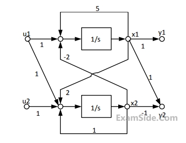
In the signal flow diagram given in the figure, $${u_1}$$ and $${u_2}$$ are possible inputs whereas $${y_1}$$ and $${y_2}$$ are possible outputs. When would the $$SISO$$ system derived from this diagram be controllable and observable?
Questions Asked from Marks 2
GATE EE 2025 (1) GATE EE 2023 (1) GATE EE 2017 Set 1 (1) GATE EE 2017 Set 2 (1) GATE EE 2016 Set 1 (1) GATE EE 2015 Set 1 (1) GATE EE 2015 Set 2 (1) GATE EE 2014 Set 3 (1) GATE EE 2014 Set 2 (1) GATE EE 2013 (2) GATE EE 2012 (1) GATE EE 2010 (1) GATE EE 2009 (2) GATE EE 2008 (2) GATE EE 2005 (2) GATE EE 2004 (1) GATE EE 2003 (1) GATE EE 2002 (2)
GATE EE Subjects
Electromagnetic Fields
Signals and Systems
Engineering Mathematics
General Aptitude
Power Electronics
Power System Analysis
Analog Electronics
Control Systems
Digital Electronics
Electrical Machines
Electric Circuits
Electrical and Electronics Measurement