The state transition matrix for the system $$\left[ {\matrix{ {\mathop {{x_1}}\limits^ \bullet } \cr {\mathop {{x_2}}\limits^ \bullet } \cr } } \right] = \left[ {\matrix{ 1 & 0 \cr 1 & 1 \cr } } \right]\left[ {\matrix{ {{x_1}} \cr {{x_2}} \cr } } \right] + \left[ {\matrix{ 1 \cr 1 \cr } } \right]u$$ is

For a system with the transfer function $$H\left( s \right) = {{3\left( {s - 2} \right)} \over {{s^3} + 4{s^2} - 2s + 1}},\,\,$$ the matrix $$A$$ in the state space form $$\mathop X\limits^ \bullet = AX + BU$$ is equal to

A second order system starts with an initial condition of $$\left( {\matrix{ 2 \cr 3 \cr } } \right)$$ without any external input. The state transition matrix for the system is given by $$\left( {\matrix{ {{e^{ - 2t}}} & 0 \cr 0 & {{e^{ - t}}} \cr } } \right).$$ The state of the system at the end of $$1$$ second is given by.

The state transition matrix for the system $$\mathop X\limits^ \bullet = AX\,\,$$ with initial state $$X(0)$$ is

Given the homogeneous state-space equation $$\mathop X\limits^ \bullet = \left[ {\matrix{ { - 3} & 1 \cr 0 & { - 2} \cr } } \right]x$$ the steady state value of $$\,\,{x_{ss}}\,\, = \mathop {Lim}\limits_{t \to \infty } x\left( t \right),$$ given the initial state value of $$x\left( 0 \right) = {\left[ {10 - 10} \right]^T},\,\,is$$

A system is described by the state equation $$\mathop X\limits^ \bullet = AX + BU$$ , The output is given by $$Y=CX$$ Where $$A = \left( {\matrix{ { - 4} & { - 1} \cr 3 & { - 1} \cr } } \right)\,\,B = \left( {\matrix{ 1 \cr 1 \cr } } \right)\,\,C = \left[ {10} \right]$$

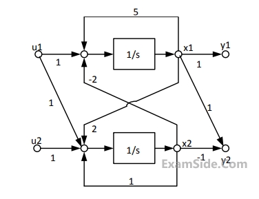
Transfer function $$G(s)$$ of the system is

The matrix of any state space equations for the transfer function $$C(s)/R(s)$$ of the system, shown below in. Figure is

The transfer function for the state variable representation $$\mathop X\limits^ \bullet = AX + BU,\,\,Y = CX + DU,$$ is given by

Consider a second order system whose state space representation is of the form $$\mathop X\limits^ \bullet = AX + BU.$$ If $$\,{x_1}\,\,\left( t \right)\, = {x_2}\,\left( t \right),$$ then system is

Consider the state-space model $$ \begin{aligned} \dot{x}(t) & =A x(t)+B u(t) \\ y(t) & =C x(t) \end{aligned} $$ where $x(t), r(t), y(t)$ are the state, input and output, respectively. The matrices $A, B, C$ are given below $$ A=\left[\begin{array}{cc} 0 & 1 \\ -2 & -3 \end{array}\right], B=\left[\begin{array}{l} 0 \\ 1 \end{array}\right], C=\left[\begin{array}{ll} 1 & 0 \end{array}\right] $$ The sum of the magnitudes of the poles is ___________. (Round off to nearest integer)

Consider the state-space description of an LTI system with matrices

$$A = \left[ {\matrix{ 0 & 1 \cr { - 1} & { - 2} \cr } } \right],B = \left[ {\matrix{ 0 \cr 1 \cr } } \right],C = \left[ {\matrix{ 3 & { - 2} \cr } } \right],D = 1$$

For the input, $$\sin (\omega t),\omega > 0$$, the value of $$\omega$$ for which the steady-state output of the system will be zero, is ___________ (Round off to the nearest integer).

Consider the system described by the following state space representation
$$\eqalign{ & \left[ {\matrix{ {\mathop {{x_1}}\limits^ \bullet \left( t \right)} \cr {\mathop {{x_2}}\limits^ \bullet \left( t \right)} \cr } } \right] = \left[ {\matrix{ 0 & 1 \cr 0 & { - 2} \cr } } \right]\left[ {\matrix{ {{x_1}\left( t \right)} \cr {{x_2}\left( t \right)} \cr } } \right] + \left[ {\matrix{ 0 \cr 1 \cr } } \right]u\left( t \right) \cr & y\left( t \right) = \left[ {\matrix{ 1 & 0 \cr } } \right]\left[ {\matrix{ {{x_1}\left( t \right)} \cr {{x_2}\left( t \right)} \cr } } \right] \cr} $$

If $$u(t)$$ is a unit step input and $$\left[ {\matrix{ {{x_1}\left( 0 \right)} \cr {{x_2}\left( 0 \right)} \cr } } \right] = \left[ {\matrix{ 1 \cr 0 \cr } } \right],$$ the value of output $$y(t)$$ at $$t=1$$ sec (rounded off to three decimal places) is _____________.

The transfer function of the system $$Y\left( s \right)/U\left( s \right)$$ , whose state-space equations are given below is:
$$\eqalign{ & \left[ {\matrix{ {\mathop {{x_1}}\limits^ \bullet \left( t \right)} \cr {\mathop {{x_2}}\limits^ \bullet \left( t \right)} \cr } } \right] = \left[ {\matrix{ 1 & 2 \cr 2 & 0 \cr } } \right]\left[ {\matrix{ {{x_1}\left( t \right)} \cr {{x_2}\left( t \right)} \cr } } \right] + \left[ {\matrix{ 1 \cr 2 \cr } } \right]u\left( t \right) \cr & y\left( t \right) = \left[ {\matrix{ 1 & 0 \cr } } \right]\left[ {\matrix{ {{x_1}\left( t \right)} \cr {{x_2}\left( t \right)} \cr } } \right] \cr} $$

Consider the following state - space representation of a linear time-invariant system.
$$\mathop x\limits^ \bullet \left( t \right) = \left[ {\matrix{ 1 & 0 \cr 0 & 2 \cr } } \right]\,\,x\left( t \right),\,\,y\left( t \right) = {c^T}x\left( t \right),\,c = \left[ {\matrix{ 1 \cr 1 \cr } } \right]$$ and
$$x\left( 0 \right) = \left[ {\matrix{ 1 \cr 1 \cr } } \right]$$

The value of $$y(t)$$ for $$t\,\,\, = \,\,{\log _e}2$$ ___________.

In the signal flow diagram given in the figure, $${u_1}$$ and $${u_2}$$ are possible inputs whereas $${y_1}$$ and $${y_2}$$ are possible outputs. When would the $$SISO$$ system derived from this diagram be controllable and observable?

For the system governed by the set of equations: $$$\eqalign{ & d{x_1}/dt = 2{x_1} + {x_2} + u \cr & d{x_2}/dt = - 2{x_1} + u \cr & \,\,\,\,\,\,y = 3{x_1} \cr} $$$
the transfer function $$Y(s)/U(s)$$ is given by

The second order dynamic system $${{dX} \over {dt}} = PX + Qu,\,\,\,y = RX$$ has the matrices $$P,Q,$$ and $$R$$ as follows: $$P = \left[ {\matrix{ { - 1} & 1 \cr 0 & { - 3} \cr } } \right]\,\,Q = \left[ {\matrix{ 0 \cr 1 \cr } } \right]$$
$$R = \left[ {\matrix{ 0 & 1 \cr } } \right]$$ The system has the following controllability and observability properties:

Consider the system described by the following state space equations $$$\eqalign{ & \left[ {\matrix{ {{x_1}} \cr {{x_2}} \cr } } \right] = \left[ {\matrix{ 0 & 1 \cr { - 1} & { - 1} \cr } } \right]\left[ {\matrix{ {{x_1}} \cr {{x_2}} \cr } } \right] + \left[ {\matrix{ 0 \cr 1 \cr } } \right]u; \cr & y = \left[ {\matrix{ 1 & 0 \cr } } \right]\left[ {\matrix{ {{x_1}} \cr {{x_2}} \cr } } \right] \cr} $$$

If $$u$$ unit step input, then the steady state error of the system is

The state variable formulation of a system is given as
$$\left[ {\matrix{ {\mathop {{x_1}}\limits^ \bullet } \cr {\mathop {{x_2}}\limits^ \bullet } \cr } } \right] = \left[ {\matrix{ { - 2} & 0 \cr 0 & { - 1} \cr } } \right]\left[ {\matrix{ {{x_1}} \cr {{x_2}} \cr } } \right] + \left[ {\matrix{ 1 \cr 1 \cr } } \right]u,\,\,{x_1}\left( 0 \right) = 0,$$
$${x_2}\left( 0 \right) = 0$$ and $$y = \left[ {\matrix{ 1 & 0 \cr } } \right]\left[ {\matrix{ {{x_1}} \cr {{x_2}} \cr } } \right]$$

The system is

The state variable formulation of a system is given as
$$\left[ {\matrix{ {\mathop {{x_1}}\limits^ \bullet } \cr {\mathop {{x_2}}\limits^ \bullet } \cr } } \right] = \left[ {\matrix{ { - 2} & 0 \cr 0 & { - 1} \cr } } \right]\left[ {\matrix{ {{x_1}} \cr {{x_2}} \cr } } \right] + \left[ {\matrix{ 1 \cr 1 \cr } } \right]u,\,\,{x_1}\left( 0 \right) = 0,$$
$${x_2}\left( 0 \right) = 0$$ and $$y = \left[ {\matrix{ 1 & 0 \cr } } \right]\left[ {\matrix{ {{x_1}} \cr {{x_2}} \cr } } \right]$$

The response $$y(t)$$ to a unit step input is

The state variable description of an $$LTI$$ system is given by $$$\left( {\matrix{ {\mathop {{x_1}}\limits^ \bullet } \cr {\mathop {{x_2}}\limits^ \bullet } \cr {\mathop {{x_3}}\limits^ \bullet } \cr } } \right) = \left( {\matrix{ 0 & {{a_1}} & 0 \cr 0 & 0 & {{a_2}} \cr {{a_3}} & 0 & 0 \cr } } \right)\left( {\matrix{ {{x_1}} \cr {{x_2}} \cr {{x_3}} \cr } } \right) + \left( {\matrix{ 0 \cr 0 \cr 1 \cr } } \right)u,$$$ $$$y = \left( {\matrix{ 1 & 0 & 0 \cr } } \right)\left( {\matrix{ {{x_1}} \cr {{x_2}} \cr {{x_3}} \cr } } \right)$$$

where $$y$$ is the output and $$u$$ is the input. The system is controllable for

The system $$\mathop X\limits^ \bullet = AX + BU$$ with $$A = \left[ {\matrix{ { - 1} & 2 \cr 0 & 2 \cr } } \right],$$ $$B = \left[ {\matrix{ 0 \cr 1 \cr } } \right]$$ is

A system is described by the following state and output equations $$${{d{x_1}\left( t \right)} \over {dt}} = - 3{x_1}\left( t \right) + {x_2}\left( t \right) + 2u\left( t \right)$$$ $$${{d{x_2}\left( t \right)} \over {dt}} = - 2{x_2}\left( t \right) + u\left( t \right)$$$

$$y\left( t \right) = {x_1}\left( t \right)$$ when $$u(t)$$ is the input and $$y(t)$$ is the output

The system transfer function is

A system is described by the following state and output equations $$${{d{x_1}\left( t \right)} \over {dt}} = - 3{x_1}\left( t \right) + {x_2}\left( t \right) + 2u\left( t \right)$$$ $$${{d{x_2}\left( t \right)} \over {dt}} = - 2{x_2}\left( t \right) + u\left( t \right)$$$

$$y\left( t \right) = {x_1}\left( t \right)$$ when $$u(t)$$ is the input and $$y(t)$$ is the output

The state $$-$$ transition matrix of the above system is

The state space equation of a system is described by $$\mathop X\limits^ \bullet = AX + BU,\,\,Y = Cx$$ where $$X$$ is state vector, $$U$$ is input, $$Y$$ is output and $$$A = \left( {\matrix{ 0 & 1 \cr 0 & { - 2} \cr } } \right)\,\,B = \left( {\matrix{ 0 \cr 1 \cr } } \right)\,\,C = \left[ {\matrix{ 1 & 0 \cr } } \right]$$$

The transfer function $$G(s)$$ of this system will be

The state space equation of a system is described by $$\mathop X\limits^ \bullet = AX + BU,\,\,Y = Cx$$ where $$X$$ is state vector, $$U$$ is input, $$Y$$ is output and $$$A = \left( {\matrix{ 0 & 1 \cr 0 & { - 2} \cr } } \right)\,\,B = \left( {\matrix{ 0 \cr 1 \cr } } \right)\,\,C = \left[ {\matrix{ 1 & 0 \cr } } \right]$$$

A unity feedback is provided to the above system $$G(s)$$ to make it a closed loop system as shown in figure.

For a unit step input $$r(t),$$ the steady state error in the input will be

A state variable system
$$\mathop X\limits^ \bullet \left( t \right) = \left( {\matrix{ 0 & 1 \cr 0 & { - 3} \cr } } \right)X\left( t \right) + \left( {\matrix{ 1 \cr 0 \cr } } \right)u\left( t \right)$$ with the initial condition $$X\left( 0 \right) = {\left[ { - 1\,\,3} \right]^T}$$ and the unit step input $$u(t)$$ has

The state transition matrix

A state variable system
$$\mathop X\limits^ \bullet \left( t \right) = \left( {\matrix{ 0 & 1 \cr 0 & { - 3} \cr } } \right)X\left( t \right) + \left( {\matrix{ 1 \cr 0 \cr } } \right)u\left( t \right)$$ with the initial condition $$X\left( 0 \right) = {\left[ { - 1\,\,3} \right]^T}$$ and the unit step input $$u(t)$$ has

The state transition equation

The state variable description of a linear autonomous system is, $$\mathop X\limits^ \bullet = AX,\,\,$$ where $$X$$ is the two dimensional state vector and $$A$$ is the system matrix given by $$A = \left[ {\matrix{ 0 & 2 \cr 2 & 0 \cr } } \right].$$ The roots of the characteristic equation are

The following equation defines a separately exited $$dc$$ motor in the form of a differential equation $${{{d^2}\omega } \over {d{t^2}}} + {{B\,d\omega } \over {j\,\,dt}} + {{{K^2}} \over {LJ}}\omega = {K \over {LJ}}{V_a}$$

The above equation may be organized in the state space form as follows
$$\left( {\matrix{ {{{{d^2}\omega } \over {d{t^2}}}} \cr {{{d\omega } \over {dt}}} \cr } } \right) = P\left( {\matrix{ {{{d\omega } \over {dt}}} \cr \omega \cr } } \right) + Q{V_a}$$

where the $$P$$ matrix is given by

For the system $$\mathop X\limits^ \bullet = \left[ {\matrix{ 2 & 0 \cr 0 & 4 \cr } } \right]X + \left[ {\matrix{ 1 \cr 1 \cr } } \right]u;\,\,\,y = \left[ {\matrix{ 4 & 0 \cr } } \right]X,\,$$ with u as unit impulse and with zero initial state, the output, $$y$$, becomes

For the system $$X = \left[ {\matrix{ 2 & 3 \cr 0 & 5 \cr } } \right]X + \left[ {\matrix{ 1 \cr 0 \cr } } \right]u,$$ Which of the following statement is true?

Obtain a state variable representation of the system governed by the differential equation: $${{{d^2}y} \over {d{t^2}}} + {{dy} \over {dt}} - 2y = u\left( t \right){e^{ - t}},\,\,\,$$ with the choice of state variables as $${x_1} = y,$$ $${x_2} = \left( {{{dy} \over {dt}} - y} \right){e^t}.$$ Aso find $${x_2}\left( t \right),$$ given that $$u(t)$$ is a unit step function and $${x_2}\left( 0 \right) = 0.$$

Consider the state equation $$\mathop X\limits^ \bullet \left( t \right) = Ax\left( t \right)$$
Given : $${e^{AT}} = \left[ {\matrix{ {{e^{ - t}} + t{e^{ - t}}} & {t{e^{ - t}}} \cr { - t{e^{ - t}}} & {{e^{ - t}} - t{e^{ - t}}} \cr } } \right]$$

(a) Find a set of states $${x_1}\left( 1 \right)$$ and $${x_2}\left( 1 \right)$$ such that $${x_1}\left( 2 \right) = 2.$$
(b) Show that $$\,{\left( {s{\rm I} - A} \right)^{ - t}} = \Phi \left( s \right) = {1 \over \Delta }\left[ {\matrix{ {s + 2} & 1 \cr { - 1} & s \cr } } \right];$$ $$\Delta = {\left( {s + 1} \right)^2}$$
(c) From $$\Phi \left( s \right),$$ find the matrix $$A$$.

The state-space representation of a system is given by $$\left[ {\matrix{ {\mathop {{X_1}}\limits^ \bullet } \cr {\mathop {{X_2}}\limits^ \bullet } \cr } } \right] = \left[ {\matrix{ { - 5} & 1 \cr { - 6} & 0 \cr } } \right]\left[ {\matrix{ {{x_1}} \cr {{x_2}} \cr } } \right].$$
Find the Laplace transform of the state transistion matrix. Find also the value of $${x_1}$$ at $$t=1$$ if $${x_1}\left( 0 \right) = 1$$ and $${x_2}\left( 0 \right) = 0.$$

Determine the transfer function of the system having the following state variable representation:
$$\eqalign{ & X = \left[ {\matrix{ 0 & 1 & 0 \cr 0 & 0 & 1 \cr { - 40} & { - 44} & { - 14} \cr } } \right]x + \left[ {\matrix{ 0 \cr 1 \cr 0 \cr } } \right]u \cr & y = \left[ {\matrix{ 0 & 1 & 0 \cr } } \right]x \cr} $$